
AI Inference Cost Optimization: The Complete Guide to Running AI Cheaper and Faster in Production

Every engineering team that ships a model into production eventually hits the same wall. Training was the fun part — the experimentation, the benchmark chasing, the model card. Then the bill for serving that model to real users arrives, and it doesn't stop arriving. AI inference cost optimization is the discipline that decides whether your AI product has a sustainable unit economics story or a slow-motion budget crisis, and in 2026 it's arguably the single most consequential skill an AI infrastructure team can develop.
This guide walks through the full stack, layer by layer, with the math you need to actually calculate your cost per token — not just intuit that "smaller models are cheaper."
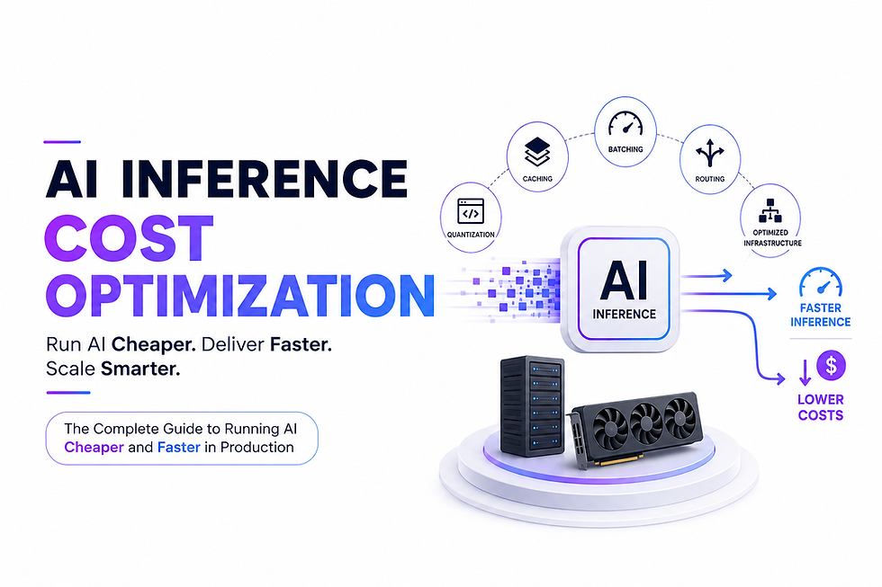
What is AI inference cost optimization?
It is the system-level engineering process of reducing GPU compute expense, memory footprint, and token-level latency — measured through Time to First Token (TTFT) and Time per Output Token (TPOT) — while holding output accuracy within an agreed SLA. It spans five interconnected layers: prompt design, model compression, the serving runtime, hardware selection, and orchestration logic. Teams that treat these as one system rather than five separate problems tend to be the ones who cut serving costs by an order of magnitude without users noticing a thing.
Here's the uncomfortable part most roadmaps skip over. Training a foundation model is a one-time capital expense. Inference is the recurring operational expense that scales linearly — sometimes worse — with every new user, every new session, every new agentic loop your product runs. Industry cost breakdowns from GPU cloud providers and infrastructure teams consistently put inference at 80% to 90% of total lifecycle AI spend for any product past its first few months in production. That's the paradox: the phase that gets the least engineering attention during the build phase becomes the phase that determines whether the product is actually profitable.
Understanding the AI Inference Bottleneck: Memory Bandwidth vs. Compute
The Anatomy of an LLM Call: Prefill vs. Decode Phases
Every LLM inference call runs through two structurally different phases, and conflating them is where most cost-optimization strategies go wrong.
The prefill phase happens when the model reads your entire input prompt and builds the initial KV cache in a single parallel pass. This phase is compute-bound — the GPU's tensor cores are the bottleneck, not memory movement, because the model processes all input tokens simultaneously as one large matrix multiplication. Long prompts, large RAG contexts, and lengthy system instructions all inflate this phase directly.
The decode phase is different in kind, not just degree. Once generation starts, the model produces one token at a time, and each new token requires reading the entire KV cache back from GPU memory. This phase is memory-bandwidth-bound — the GPU's compute cores sit mostly idle, waiting on data to arrive from HBM. This is why a GPU with more raw FLOPS doesn't automatically make decoding faster; what matters is how fast the memory subsystem can feed the compute units.
Time to First Token (TTFT) vs. Time per Output Token (TPOT)
TTFT measures how long a user waits before seeing the first character of a response — it's almost entirely a function of prefill efficiency and prompt length. TPOT measures the per-token generation speed once streaming begins — it's a function of memory bandwidth, batch density, and KV cache management.
This distinction matters operationally because the fixes are different. Reducing TTFT means shrinking or compressing the input context. Reducing TPOT means better memory management, quantization, and batching — attacking the input side won't fix a slow decode loop, and attacking the decode loop won't fix a bloated context window.
Key Metrics That Drive Your Inference Bill
Four numbers determine almost everything about your serving cost:
VRAM footprint — model weights plus KV cache plus activation memory, all competing for the same finite GPU memory pool
Memory bandwidth (TB/s) — how fast the GPU can move KV cache data during decode
Batch size density — how many concurrent requests you can pack into the same GPU memory without OOM errors
GPU utilization percentage — the gap between theoretical FLOPS and what your actual workload achieves, which is often shockingly low without runtime-level optimization
The FourfoldAI 5-Layer Inference Optimization Pyramid
At FourfoldAI, we think about inference cost as a pyramid rather than a checklist, because each layer changes what's achievable in the layer above it. Fixing one layer in isolation produces marginal gains. Fixing all five in sequence produces compounding ones.
Layer 1 — Prompt & Context Level: This is where you control what actually reaches the model. Semantic caching, context trimming, and prefix reuse reduce the raw volume of tokens the GPU has to process before generation even starts.
Layer 2 — Model Architecture & Compression Level: Quantization, distillation, and pruning shrink the model itself, reducing both the VRAM it occupies and the compute required per forward pass.
Layer 3 — Serving Engine & Memory Runtime Level: This is where PagedAttention, continuous batching, chunked prefill, and speculative decoding determine how efficiently your hardware is actually used moment to moment.
Layer 4 — Hardware & Compute Infrastructure Level: GPU selection and provisioning strategy — matching VRAM and bandwidth profiles to your actual workload instead of over-provisioning out of habit.
Layer 5 — System Orchestration & Dynamic Routing Level: The macro layer, where you decide which requests even need your most expensive model in the first place.
The order matters. A team that jumps straight to buying B200 clusters before fixing their prompt bloat and batching strategy is solving the wrong problem first.
Layer 1 — Prompt & Context Optimization
Semantic Caching: Avoiding Redundant Model Execution
A large share of production traffic — especially in support, search, and internal tooling contexts — consists of semantically identical or near-identical queries phrased differently. Semantic caching stores embeddings of previous queries in a vector index (Qdrant, Redis with vector search, or similar) and checks incoming requests against that index before touching the LLM at all. A cache hit means zero GPU inference cost for that request. This is the single highest-leverage optimization available before you touch the model or the runtime, because it eliminates compute entirely rather than making it cheaper.
Prompt Compression & Context Trimming
Not every token in a prompt carries equal information density. Techniques like LLMLingua and selective-context filtering identify and strip low-information tokens — filler phrasing, redundant instructions, boilerplate — before the prompt reaches the model. Because the prefill phase is compute-bound and scales with input length, trimming a bloated 4,000-token system prompt down to 1,200 meaningful tokens directly reduces TTFT and lowers the compute cost of every single call built on that template.
Prefix Caching for Multi-Turn Conversations & System Prompts
Multi-turn conversations and agentic loops repeat the same system prompt and conversation history on every turn. Prefix caching stores the KV cache for the shared prefix once and reuses it across subsequent calls instead of recomputing it from scratch each time. For chat applications with long, stable system prompts, this alone can cut prefill compute dramatically on turn two and beyond.

Layer 2 — Model Compression: Quantization, Distillation & Pruning
Quantization Deep Dive: FP16 vs. FP8 vs. INT4 / AWQ vs. GPTQ
Quantization reduces the numerical precision used to store model weights (and sometimes activations), trading a small amount of accuracy for large gains in memory footprint and throughput. Weight-only quantization (like GPTQ and AWQ) compresses stored weights while keeping activations at higher precision during computation — a safer, more broadly compatible approach. Weight-and-activation quantization (like FP8) compresses both, unlocking larger throughput gains on hardware with native low-precision tensor cores, which is exactly what Hopper and Blackwell architectures are built around.
AWQ (Activation-aware Weight Quantization) is notable because it doesn't quantize all weights equally — it identifies which weight channels matter most for preserving activation quality and protects them, which is why it tends to hold accuracy better than naive round-to-nearest quantization at the same bit width.
Quantization Scheme | VRAM Reduction | Latency Impact | Accuracy Loss | Best Production Use Case |
FP8 | ~50% vs. FP16 | Low latency impact; near-native throughput on Hopper/Blackwell tensor cores | Minimal (near-lossless on most benchmarks) | High-throughput production serving on H100/H200/B200 |
AWQ (INT4) | ~65-75% vs. FP16 | Moderate speedup; strong on memory-bound decode | Low-to-moderate, protects salient weight channels | Cost-sensitive deployment of 13B-70B models on limited VRAM |
GPTQ (INT4) | ~65-75% vs. FP16 | Moderate speedup, calibration-dependent | Low-to-moderate, sensitive to calibration dataset quality | Offline-calibrated deployments where calibration data is representative |
GGUF (INT4/INT5/INT8 mixed) | Variable, highly configurable | Strong on CPU and consumer GPU / Apple Silicon | Configurable trade-off by quant level | Local inference, edge deployment, llama.cpp-based serving |
EXL2 | Variable, mixed-bit per layer | Fast on consumer GPUs | Low, mixed-precision allocation improves quality retention | Single-GPU consumer/prosumer inference workloads |
The practical rule of thumb: FP8 is usually the safest first move for production LLMs on modern NVIDIA hardware because the accuracy loss is typically negligible while the throughput gain is substantial. INT4 methods like AWQ and GPTQ go further on VRAM savings but require more careful evaluation against your specific task before shipping — particularly for reasoning-heavy workloads, which brings us to one of the most common production mistakes covered later in this guide.
Knowledge Distillation: Replacing 70B Models with Specialized 8B/3B SLMs
Distillation trains a smaller "student" model to mimic the outputs of a larger "teacher" model on a specific task distribution. Instead of running a general-purpose 70B model for every request, teams increasingly distill task-specific behavior into 8B or even 3B small language models (SLMs). For narrow, well-defined tasks — classification, extraction, routing decisions, templated summarization — a well-distilled small model can match teacher-level accuracy on that specific task while running at a fraction of the inference cost and latency.
Structural Pruning and MoE Sparse Execution
Structural pruning removes entire redundant components — attention heads, layers, or neuron blocks — from a trained model, rather than just reducing numerical precision. It's a more invasive optimization that requires fine-tuning afterward to recover accuracy, but it directly reduces the FLOPs required per forward pass.
Mixture-of-Experts architecture takes a different approach to the same goal: sparsity by design rather than by removal. DeepSeek-V3, for example, holds 671 billion total parameters but activates only 37 billion per token, routing each token through a small subset of specialized expert sub-networks instead of the full parameter set. The practical effect is that you get frontier-scale model capacity while paying compute costs closer to what a 37B dense model would cost — this is precisely why MoE architectures have become the default design pattern for cost-conscious frontier labs rather than a niche technique.
Layer 3 — Serving Engines & Memory Runtime Optimization
This is where most of the engineering leverage in production inference actually lives, and it's the layer most teams under-invest in relative to its impact.
PagedAttention and KV Cache Management
Before PagedAttention, serving systems allocated a large contiguous block of GPU memory for each request's KV cache, sized for the maximum possible sequence length. Because actual generated sequences are almost always shorter than the worst case, this pre-allocation wasted enormous amounts of VRAM to internal fragmentation — memory reserved but never used.
PagedAttention, introduced by the UC Berkeley Sky Computing Lab and implemented in the vLLM serving engine, borrows the paging concept from operating system virtual memory. Instead of one contiguous block per request, the KV cache is split into fixed-size blocks that can be allocated non-contiguously and shared flexibly across requests. The original vLLM research demonstrated near-zero waste in KV cache memory and throughput improvements of several multiples over prior serving systems on the same hardware, because far more concurrent requests fit into the same VRAM pool.
The downstream effect on cost is direct: more concurrent requests per GPU means more tokens generated per GPU-hour, which is the denominator in every inference cost equation.
Continuous Batching (Iteration-Level Scheduling)
Legacy static batching groups a fixed set of requests together and waits for the entire batch to finish generating before accepting new requests — meaning a single long-running request holds up GPU capacity that shorter, already-finished requests could otherwise be using. Continuous batching (also called iteration-level scheduling) evaluates the batch at every generation step, immediately slotting in new requests as soon as any sequence in the current batch completes. This keeps GPU utilization consistently high instead of oscillating between full and idle, and it's one of the core innovations that made modern high-throughput serving engines dramatically more efficient than naive batch inference loops.
Speculative Decoding: Draft Models & Parallel Verification
Speculative decoding attacks the memory-bandwidth bottleneck of the decode phase directly. A small, fast "draft" model (for example, a 1B-parameter model) proposes several candidate tokens ahead of the main generation, and the larger "target" model (say, a 70B model) verifies those candidate tokens in a single parallel forward pass rather than generating them one at a time sequentially. When the draft model's guesses are accepted — which happens often for predictable text — you get multiple tokens' worth of output for roughly the cost of one target-model forward pass. In practice, well-tuned speculative decoding setups commonly deliver meaningful TPOT improvements, though the exact multiplier depends heavily on how well the draft model's output distribution matches the target model's on your specific traffic.
Benchmark Comparison: vLLM vs. TensorRT-LLM vs. SGLang vs. TGI
Serving Engine | TTFT Characteristics | TPOT Characteristics | Memory Efficiency | Setup Complexity | Recommended Use Case |
vLLM | Strong, PagedAttention-driven | Strong under high concurrency | Very high — near-zero KV cache waste | Low-to-moderate, broad model support | General-purpose production serving, fastest path from Hugging Face model to endpoint |
TensorRT-LLM | Very strong on NVIDIA hardware after compilation | Very strong with FP8/INT4 kernel fusion | High, NVIDIA-optimized kernels | Higher — requires engine compilation per model/GPU config | Latency-critical NVIDIA-only deployments at scale |
SGLang | Strong, especially with RadixAttention prefix sharing | Strong, efficient structured output generation | High, radix-tree-based KV cache reuse | Moderate | Workloads with heavy prompt reuse, structured/JSON output, agentic pipelines |
TGI (Text Generation Inference) | Solid, Hugging Face-native | Solid | Moderate-to-high | Low, tightly integrated with HF ecosystem | Teams already standardized on Hugging Face tooling |
The honest answer to "which is fastest" is that it depends on your model, hardware, and traffic shape more than any single benchmark number. vLLM tends to win on ease of adoption and broad model compatibility. TensorRT-LLM tends to win on raw latency once you've invested in the compilation step for a fixed model and GPU configuration. SGLang's RadixAttention design gives it a distinct edge for workloads with heavy prompt-prefix reuse and structured output generation, which is increasingly the dominant pattern in agentic and tool-calling systems.
Layer 4 — Hardware & Compute Provisioning
GPU Selection Matrix: Matching Hardware to Workload Profile
GPU | VRAM | Memory Bandwidth | Best Fit |
NVIDIA L40S | 48 GB | Lower bandwidth than data-center Hopper cards | Cost-efficient inference for models under ~13B, lighter concurrency |
NVIDIA H100 | 80 GB HBM3 | ~3.35 TB/s | Workhorse for models up to ~34B where 80GB is sufficient, compute-bound tasks |
NVIDIA H200 | 141 GB HBM3e | ~4.8 TB/s | Large-context inference, 70B-class models needing more headroom without multi-GPU sharding |
NVIDIA B200 (Blackwell) | 180 GB HBM3e | ~8 TB/s, native FP4/FP8 support | Frontier-scale MoE models, highest-throughput production inference |
AMD Instinct MI300X | 192 GB HBM3 | High bandwidth, ROCm-based stack | Teams optimizing for memory capacity per dollar outside the NVIDIA/CUDA ecosystem |
The mistake we see most often here is provisioning by "biggest available GPU" rather than by workload profile. If your model and KV cache comfortably fit in 80GB, an H100 frequently delivers a better cost-per-token than an H200 or B200, because you're not paying a premium for memory bandwidth headroom you never use. The upgrade to H200 or B200 pays for itself specifically when your model, context length, or concurrency target pushes past what an H100 can hold — not as a default choice.
Serverless vs. Dedicated Instance Economics
Serverless inference endpoints (Together AI, Groq, Fireworks, and similar providers) charge per token and abstract away all provisioning decisions — ideal for unpredictable or low-volume traffic where idle GPU time on a dedicated cluster would otherwise be pure waste. Self-hosted deployment on vLLM running on managed Kubernetes (AWS EKS, GCP GKE) becomes economically favorable once your sustained throughput is high and predictable enough that the effective per-token cost of owned or reserved capacity undercuts the serverless markup — which, for most production-scale workloads, tends to happen faster than teams expect.
Multi-GPU Parallelism: Tensor Parallelism (TP) vs. Pipeline Parallelism (PP)
Tensor parallelism splits individual layers across multiple GPUs, so each GPU computes a portion of every matrix multiplication — this reduces per-GPU memory pressure but requires fast interconnect (NVLink) between GPUs since they must communicate on every layer. Pipeline parallelism instead assigns different layers of the model to different GPUs, passing activations forward through the pipeline — this tolerates slower interconnects better but can introduce pipeline bubbles that hurt utilization if not carefully scheduled. For inference specifically, tensor parallelism is generally preferred when NVLink bandwidth is available, since it keeps per-token latency lower than pipeline approaches.
Layer 5 — Orchestration & Dynamic Model Routing
Cascading Model Routers (SLM-First Architecture)
Not every query needs your most expensive model. A cascading router evaluates incoming requests — often with a lightweight classifier or the request's own complexity signals — and routes simple queries to small, cheap models while escalating genuinely complex requests to larger reasoning models. A support-ticket triage query doesn't need the same model as a multi-step financial analysis task, and treating them identically means systematically overpaying on the easy majority of your traffic to marginally improve the hard minority.
Fallback Gates & SLA-Driven Circuit Breakers
Production routing systems need circuit breakers: if the small model's confidence is low, or its output fails a validation check, the request automatically escalates to the larger model rather than returning a degraded answer. This keeps the cost savings of SLM-first routing without silently sacrificing quality on the requests that actually need more capability.
Calculating Your True Inference Cost: The Math Behind the Token
The foundational formula for token economics is straightforward once you have real throughput numbers from your own load testing:
Cost per 1M Tokens = (Hourly GPU Cost ÷ Tokens Generated per Hour) × 1,000,000
The variable that actually moves this number is Tokens Generated per Hour, and that's precisely what every layer of this guide is designed to increase — through better batching density, faster memory access, smaller active parameter counts, and fewer redundant calls reaching the model at all.
Consider a directional example. An unoptimized Llama-70B deployment running on naive batching, FP16 precision, and no prompt compression might land somewhere around $12.00 per 1M tokens on a given GPU configuration, purely because low concurrency and memory fragmentation leave most of the GPU's theoretical throughput unused. Apply the full stack — FP8 quantization, PagedAttention-based continuous batching through vLLM, speculative decoding, semantic caching that deflects a meaningful share of redundant calls, and SLM-first routing that offloads simple queries entirely — and that same workload can realistically land closer to $0.85–$1.50 per 1M tokens, depending on traffic mix and how much of it the router successfully deflects to smaller models.
That gap is not a rounding error. It's the difference between an AI feature that scales sustainably and one that gets quietly pulled from the roadmap when the finance team sees the cloud bill.
Common Pitfalls & Mistakes in Production Inference
Over-quantizing reasoning models. Aggressive INT4 quantization can be nearly lossless for straightforward extraction or classification tasks, but chain-of-thought and multi-step reasoning workloads are often far more sensitive to precision loss, since small numerical errors compound across reasoning steps. Test quantized reasoning models against your actual evaluation suite, not just generic benchmark scores.
Ignoring KV cache OOM errors under high concurrency. Systems that work fine in staging with a handful of concurrent requests can hit memory ceilings in production when concurrency spikes, especially with long-context requests. Load-test at realistic — and peak — concurrency, not average concurrency.
Neglecting prefill latency during long-context RAG. Teams optimize decode-phase throughput and forget that a 20,000-token retrieved context makes TTFT the dominant user-facing latency, not TPOT. If your product does heavy RAG, prompt compression and prefix caching deserve at least as much attention as your quantization strategy.
Frequently Asked Questions
What is AI inference cost optimization? AI inference cost optimization is the system-level engineering discipline of reducing hardware costs, VRAM consumption, and latency (TTFT and TPOT) when serving AI models in production. It combines prompt compression, quantization, memory-efficient serving runtimes like vLLM, speculative decoding, and dynamic model routing to cut cost while preserving accuracy SLAs.
What is the difference between TTFT and TPOT in LLM inference? TTFT (Time to First Token) measures how long a user waits for the first token, driven by the compute-bound prefill phase and prompt length. TPOT (Time per Output Token) measures the speed of subsequent tokens during the memory-bandwidth-bound decode phase, driven by KV cache size and memory bandwidth.
How does quantization reduce AI inference costs? Quantization lowers the numerical precision of model weights (and sometimes activations), such as moving from FP16 to FP8 or INT4. This shrinks VRAM footprint and increases throughput on hardware with native low-precision tensor cores, at the cost of a typically small, measurable accuracy trade-off.
Which serving engine is faster: vLLM or TensorRT-LLM? It depends on the workload. TensorRT-LLM often achieves the lowest raw latency on NVIDIA hardware after model-specific compilation, while vLLM offers strong throughput with far simpler setup and broader model compatibility, making it the more practical default for most teams.
What is speculative decoding in LLMs? Speculative decoding uses a small, fast draft model to propose multiple candidate tokens ahead of generation, which a larger target model then verifies in a single parallel pass. When candidate tokens are accepted, this reduces the number of sequential decode steps needed, improving TPOT.
How does PagedAttention reduce GPU VRAM usage? PagedAttention manages the KV cache in fixed-size, non-contiguous memory blocks instead of large pre-allocated contiguous blocks, similar to virtual memory paging in operating systems. This eliminates internal memory fragmentation and allows far more concurrent requests to fit into the same GPU memory.
What is semantic caching in AI applications? Semantic caching stores vector embeddings of prior queries and checks new requests against that index for meaning-level matches, not just exact text matches. A cache hit returns a stored response without invoking the model at all, eliminating inference cost for that request entirely.
How can dynamic model routing lower enterprise AI costs? Dynamic model routing evaluates each incoming request and sends simple queries to small, cheap models while escalating complex queries to larger, more expensive models. This SLM-first cascading approach avoids paying frontier-model prices for the large share of traffic that a smaller model can already handle correctly.
Conclusion & Engineering Takeaways
AI inference cost optimization isn't a single switch you flip — it's an iterative engineering discipline that spans prompt design, model compression, serving runtime, hardware selection, and orchestration logic. The teams getting this right aren't necessarily the ones with the biggest GPU budgets; they're the ones treating these five layers as one connected system, where a win in prompt compression makes quantization more effective, and better batching makes hardware provisioning decisions clearer.
Start by measuring your actual TTFT, TPOT, and cost-per-1M-tokens baseline before optimizing anything — you can't improve what you haven't measured. Then work through the layers in order: cut redundant tokens first, compress the model second, upgrade the runtime third, right-size the hardware fourth, and route intelligently last.
If you're building out your own inference stack and want deeper technical breakdowns on model evaluation, agentic architectures, or enterprise AI ROI frameworks, explore more research and guides at FourfoldAI.com.
Disclaimer:
This article is intended for informational and educational purposes only. While every effort has been made to verify technical accuracy against publicly available documentation and research at the time of writing, GPU pricing, benchmark figures, and framework capabilities change rapidly and should be independently verified before making production infrastructure decisions. For full details, see our disclaimer at fourfoldai.com/disclaimer.
References
vLLM Project — PagedAttention Design Documentation: docs.vllm.ai
Kwon et al., "Efficient Memory Management for Large Language Model Serving with PagedAttention," SOSP 2023: arxiv.org/abs/2309.06180
UC Berkeley Sky Computing Lab — vLLM Project Page: sky.cs.berkeley.edu/project/vllm
DeepSeek-AI, "DeepSeek-V3 Technical Report": arxiv.org/abs/2412.19437
NVIDIA H100/H200/B200 Specification Comparisons: baseten.co/blog/h100-vs-h200-vs-b200
SGLang Project Documentation and RadixAttention Architecture: github.com/sgl-project/sglang
About the Author
Muizz Shaikh is an AI enthusiast and digital technology professional at FourfoldAI. He is passionate about exploring AI tools, industry trends, and practical applications of emerging technologies. Through FourfoldAI, Muizz contributes to simplifying artificial intelligence for businesses and learners. Connect with him on LinkedIn: linkedin.com/in/muizz-shaikh-45b449403/
© 2026 FourfoldAI. All rights reserved.


Comments